
In the last few posts, we have shown some techniques for predicting nominal returns and real returns. We have also looked at simulating safe withdrawal rates in retirement with various stock / treasury bond allocations and lengths of retirement. Now it is time to put all of this together and develop a model for predicting the maximum safe withdrawal rate for retirement based on current market conditions. We essentially want to know how much we will need to have saved given the current state of the market and future expected returns.
Figure 1 shows the correlation of safe withdrawal rate with real returns. This scenario is for a 30 year retirement with a 80% stock / 20% bond allocation. As you can see, the correlation is quite strong between a linear model that predicts safe withdrawal rate using real returns for the next 10 years (annualized), and the actual safe withdrawal rate you can take in retirement without the portfolio reaching zero before the 30 year time period is up. The correlation between the two is an R2 of 0.84. The reason that the correlation between 10 year future return and a 30 year retirement portfolio is so high, is because the first 10 years of retirement have an outsized effect on the entire retirement, as I explained in a previous post where I talked about the sequence of returns risk in retirement portfolios.

Given that we have a model which is decent at predicting real returns using the equity allocation of investors and the inverse of the 10 year treasury bond yield (1/GS10) we should reasonably be able to predict the maximum safe withdrawal rate that can be utilized in retirement. Figure 2 shows the model fit for a 80% stocks / 20% bond allocation for a 30 year retirement. As you can see, the fit is excellent, but there is a problem. The model is giving rather odd future predictions. It is giving a maximum safe withdrawal rate currently of 2%. This is probably far too low, since the worst year ever, historically speaking, was 1966, and the safe withdrawal rate in that year only fell to 3.7%. That was a particularly bad year to retire because the following decade would be marked by high inflation and poor economic growth (stagflation) – a double whammy on a retirement portfolio. Further, the high inflation even continued into the next decade, once the growth started to normalize.
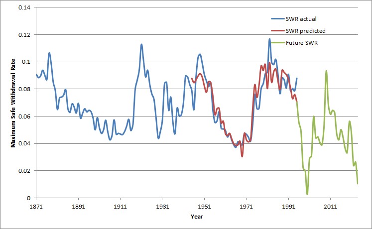
While the market is richly valued today, there is no such indication of awful inflation on the horizon, and there were times in the past with similar high valuations in the market that did not have such low safe withdrawal rates. So why are we seeing this behavior from the model? I think this is a case of the model being able to overfit the data. The more free parameters in your model, the more data you will need to fit to know that you are not overfitting spurious situations. One big clue is that the model fits the 1966-1970 region very well when there is absolutely no indication that such an awful period of stagflation was approaching based purely on looking at bond yields and equity allocation of investors – neither were particularly remarkable at this time.
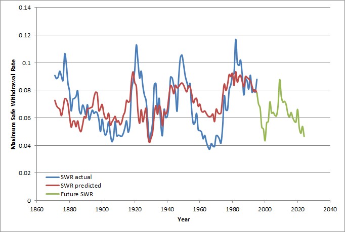
So what is to be done about this? We need more data to fit, of course. However, the equity allocation of investors data only goes back to late 1945. Nevertheless, in this previous post, I was able to derive the equity allocation of investors all the way back to 1871 using the available data from Robert Shiller. This reverse engineered data for equity allocation of investors can be used to fit the data all the way back to 1871 for equity allocation of investors based on the nominal 10 year return in the market that was realized in the subsequent 10 years. When we do this, we get a much more sensible fit, shown in Figure 3 (the correlation coefficent, R2, is 0.62). As you can see from this figure, the current prediction for maximum safe withdrawal rate is a more realistic 4.6%. Even now with a fairly high equity allocation of investors suggesting relatively lower future 10 year market returns, the prediction is still not as bad as what occurred in 1966. As the late 1960’s show, future stagflation and high inflation are retirement portfolio killers, if you aren’t careful.
Now, we have a model which can predict maximum safe withdrawal rates, but there is another problem. We are ok with underpredicting the maximum safe withdrawal rate, but we really don’t want to overpredict the maximum safe withdrawal rate, since our retirement portfolio will prematurely fall to zero if we do. We would be ok with having a bit extra at the end of retirement, but falling short and having our retirement portfolio fail early would be a disaster. So, we won’t try to find the best fit model by minimizing variance (which gives about a 50% chance of ending up short by the end of retirement), but instead we will try to build a model that under no circumstances will overpredict the safe withdrawal rate. We will accept additional error and withdraw less than we maybe could have (but still in many cases more than the hard and fast 4% rule), so long as we get to withdraw a safe amount that the market conditions will allow. We do this by adding a large penalty for fitting in any way that overpredicts the maximum safe withdrawal rate. Figure 4 shows an example of this for a 30 year retirement and an 80% stocks / 20% bonds allocation. This model still follows the data well, but never predicts a maximum safe withdrawal rate that is higher than the actual safe withdrawal rate.

However, there is still a bit more we can do. Because we force the model to fit a lower envelope of possible maximum safe withdrawal rates, this model makes some predictions that are quite low – below the lowest historical maximum safe withdrawal rate of 3.7% in the worst year (1966). This is not due to overfitting this time, but is instead due to the model being forced downward to fit the lower side of possible values. For example, currently, as of 2024, this form of the model would predict a safe withdrawal rate of 2.1%. If we are willing to accept that our risk of portfolio failure will never be zero, and that we are always taking some risk, perhaps we can live with taking a small, but reasonable risk. In this case, we can set the model to always at least predict a safe withdrawal rate that is no lower than the lowest ever observed safe withdrawal rate for that particular portfolio composition and retirement length. In only one year, 1966 out of about 125 years for which we have data, we observed this rate, so we estimate the odds of an even worse year at less than 1%. This should be a reasonable tradeoff for most people to make.
Now, we can fit the model to the lower envelope of possible maximum safe withdrawal rates, while still having a floor safe withdrawal rate of the worst year ever, historically. This allows the model to fit better and give us more situations where we can utilize a higher safe withdrawal rate if the market conditions happen to favor it (such as very undervalued markets or markets in which equity allocation to investors is very low, portending high future returns). Figure 5 shows the model fit for a 30 year retirement and an 80% stocks / 20% bonds allocation. This model fit predicts using at least a 3.7% safe withdrawal rate at all times. In a slight majority of time periods it predicts that one can use a safe withdrawal rate above 4% based on market conditions. The largest safe withdrawal rate this model has ever predicted for this scenario was around 7.9%. The safe withdrawal rates in Figure 5 may not seem like they are much of an improvement over the 4% safe withdrawal rate rule, but the difference is actually massive.

For example, let’s say you need $60,000 per year in real dollars to retire on (adjusted for inflation each year after the first year). If you choose a 4% safe withdrawal rate, you must save up $1.5 million dollars to achieve this. However, if you can safely use a 6% safe withdrawal rate, you now only need to save $1 million to retire – a massive difference that can take years off of your time to retirement. Similarly, if you are able to use the 6% safe withdrawal rate on a portfolio of $1.5 million, you can now afford to spend $90,000 per year in real dollars in retirement instead of $60,000 per year based on a 4% safe withdrawal rate – a substantial increase in standard of living.
Now, let us discuss a few of the model shortcomings. For very short retirements (less than 15-20 years), there is a lot more volatility, and uncertainty than in long retirements. Of course, you can also safely withdraw at much higher rates with short retirements, also. But I would recommend building in some bonds to reduce volatility, if you, for some reason, plan a short retirement. If you plan long retirements (20 years or more), the data seem to indicate that a portfolio with a high stock allocation is better, in agreement with others who have simulated such retirement scenarios. Bond portfolios tend to be less volatile, but also have poorer real returns in the very long run, and so have lower safe withdrawal rates. Therefore, if you have enough saved for a long retirement, it is more probable that you will be able to weather the storm of volatility in stocks over many decades, and you likely would be happier with the outcome of a high stock portfolio in that case.
I have included the model parameters for the most interesting cases in Table 1 below. To calculate the current safe withdrawal rate use the following formula:
SWR = A*EAI + B*(1/GS10)1 year avg + C
where SWR is the safe withdrawal rate to use (use the minimum value in the table if the formula above predicts a value lower than the minimum value), EAI is the equity allocation of investors, (1/GS10)1 year is the the inverse of the 10 year treasury bond yield averaged over a 1 year period, and A, B, and C are constants given in the table below.

As always, when planning retirement scenarios build in the ability to adapt. If we see another period of stagflation or very high inflation, it may be prudent to safeguard your retirement nest egg by withdrawing less for a while until conditions normalize, just in case. I think also that the equity allocation of investors data can be used to build an adaptive model that tells you what you can withdraw each year, rather than setting a constant (excepting inflation adjustments) withdrawal rate over the entire duration of retirement. However, such a scenario requires a degree of flexibility for being able to control expenses, and is more difficult to plan for, since you won’t know the sequence of withdrawal rates ahead of time. Such a method may work for some people, however.
Leave a Reply