
Continuing from the last post on my favorite valuation indicator for long term market returns, the equity allocation of investors, I wanted to follow up on this with an even better model for long term market returns. This post will get somewhat technical in data analysis, so be warned.
If you look at the post by the originator (Philosophical Economics) about the equity allocation of investors as a method of measuring future market returns, there is an excellent discussion on why the measure works. In order for investors to obtain the allocation they desire of stocks, bonds, cash, etc., given the limited supply of those things, the prices must change if everyone is to reach their allocation. If no one wants to hold a particular asset, such as bonds, for example, the price of bonds will fall until finally, some group of investors somewhere will change their allocation and hold bonds, even if grudgingly in their portfolio. This is why equity allocation of investors is such a powerful predictor of future long term market returns. If investors want or must hold a certain allocation of stocks in their portfolio, given the limited supply, the price must change over time or the investors preferences must change, or both. If allocation to stocks is very high it becomes difficult to get more growth through further increased allocations to stocks, and it becomes difficult for investors to hit return targets relative to other asset classes that begin to fall in price and look more attractive.
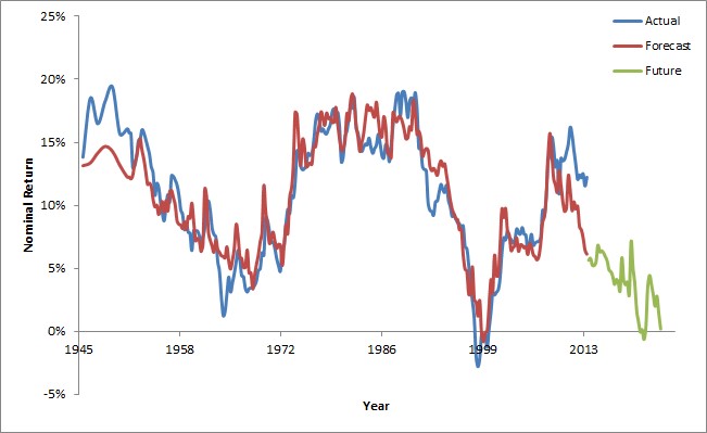
In the last post, we modeled the return as predicted by the equity allocation of investors in the market. That chart is reproduced in Figure 1 below. This model gives us pretty good predictions of the future 10 year nominal returns in the market, but can we do better? To see if we can, let us turn our focus to another interesting piece of discussion from the originator of this method.
The author of Philosophical Economics, in the same post, has an interesting discussion of valuation around the equity allocation of investors. He contends that value expectations in the market are anchored based on past behavior and that is certainly true. If the market has been at a P/E of 10 for the last 20 years, a P/E of 20 certainly looks expensive. However, if the market has been at a P/E of 30 for the last 20 years, a P/E of 20 will look like a screaming bargain.
The author contends that there is no valuation range required in the market and that values could even be a P/E of 1 or 100 if that was everyone’s expectation. I have shown in previous posts why these extremes cannot be the case over long periods of time (particularly at the lower valuations) because buying stocks at a P/E of 1 and being allowed to reinvest at such low valuations quickly lead to enormous wealth.
On the other extreme of valuation, a very high P/E of 100 is also not tenable. I have a theory that human lifetimes are tied up with minimum acceptable returns, at least at the extremes anyway. If people lived for 1000 years and retired after 900 years, they could accept a 1% annualized real return, because that would generate enormous wealth over that time period and allow them to retire. Similarly, if people lived for only 10 or 20 years, they would need returns well in excess of 20% per year to justify investing. If people live an average of 80 years as they do today, why bother investing in stocks if you can only get 1% nominal (<1% real return) at a P/E ratio of 100. You would not accumulate much real wealth over your lifetime and only your great-great-great grandchildren would start to see the results, assuming the real return is even positive after inflation. People will save and sacrifice for their own delayed benefit, for their children, and for their grandchildren, maybe even for their great-grandchildren. But after that it becomes a rather vague notion and few people plan out to such long time periods. This means probably that people have to see the fruits of their labor in timeframes on the order of 30-80 years. They will of course accept timeframes that are faster, but slower is a tough sell. So, I do not think the argument put forth by Philosophical Economics holds at extreme valuations. However, at reasonable ranges of valuation, the valuation exerts a more gentle pull, and expectations can, at least temporarily, exert a stronger pull.
To see if we can improve upon the equity allocation of investors in light of the discussion about anchoring, let us look at the residuals of the errors in the prediction vs. the return that was actually realized. The residual is just the amount by which the model over- or under-predicted the future 10 year return, and is shown in Figure 2.
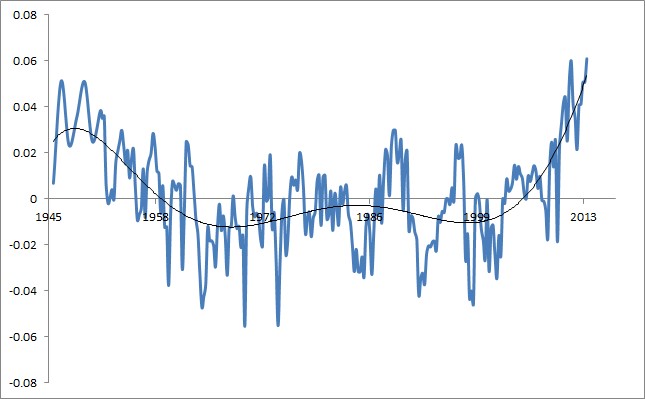
Now, it should be said that we can’t predict perfectly every up and down error in the return by simply adding more stuff to this model. There are reasons why we can’t perfectly predict things. To do so would require anticipating political events, the housing crisis, oil shocks in the 1970’s, etc. These events are shocks that are exogenous to the market, and, while blunted in impact when averaged over 10 years of market returns, still exert influence. Things that are exogenous to the market would require a model outside of the market to represent it, and we can’t build models for, or even anticipate, all the possible factors that could influence the market. So, at the very least, when we have described all of the errors possible in our model, we like to see a residual that looks flat and noisy like the one shown in Figure 3. The remaining noise is stuff we just cannot explain with our model.

If instead we see a residual that looks like Figure 4, we have a clue that perhaps something in our model is left unexplained. This is not always the case, and sometimes you simply cannot know what the unexplained portion is, so you have to accept it. But if you see something happening like in Figure 4, it is a good idea to go hunting for the explanation of the trend so you can try to incorporate this into your model. Once it is incorporated, assuming you can explain it, the residuals of the fit data will look like that in Figure 3 – random noise.

Now, let’s look at the residuals of our model for equity allocation of investors. Figure 2 shows that we have some systematic, unexplained variance. We do not see a flat, and noisy curve. This is a clue that we may be able to hunt for explanations of this unexplained systematic variance. This systematic deviation appeared to be high in the 1940’s and 50’s, low in the 1960’s – 1990’s, and high again from the mid 2000’s onward. What could be causing such a deviation? The answer is, anchored expectations of investors about what the market valuation “should” be vs. the actual valuation! If investors think the market should be lower but it is higher, they are more reluctant to buy, while if the reverse is true, they are more eager to buy. More accurately, they are more eager to allocate higher or lower fractions of their portfolio to stocks in different circumstances. While a certain equity allocation of investors has implied a particular return over 10 year periods, investors anchored higher or lower in expectation can exert a bias on this measure upwards or downwards, and that is why I think we see some systematic error in the residuals.
So now the question becomes how we figure out what those investor expectations are, but before we do that, we should understand how these anchoring behaviors occur amongst investors. Investors can change their minds slowly over time about valuation, or suddenly all at once in response to particularly salient events like the housing crash in 2008 or the Great Depression. We need some measure that can give us a good idea of the particular anchor at that moment in time.
In addition, we want to add as few parameters to our model as possible to keep it simple. Using a minimal number of parameters in our model gives less chance that we are over-fitting the data and that random fluctuations in each parameter just happen to match up with some aspect of the noise in the data. In that case, the over-fit data would have poor predictive capability going forward, since you didn’t really fit actual true phenomena, you just happened to fit the noise better by chance.
So what can we use to capture this anchored value expectation at each moment in time? I propose that we use the following measure:
[1 / GS10]1 year average
where GS10 is the yield on the 10 year bond. We use the 10 year bond because it contains expectations about the future 10 years which is the time period we are interested in. I should note that I have tested other treasury bond durations also, and most capture the same trend, some are slightly better or worse, but in the end, you can use whichever you wish. We average this over the course of a year to smooth out any sudden changes. I have tried both averaging and not averaging and they produce similar results. A 1 year average produces very slightly better results, and I like to make sure that the measure changes somewhat smoothly in the event that there are any sudden spikes or troughs of rapid change in the future.
So what precisely is this measure that we are calculating? It is essentially the P/E of a bond (inverse of yield). In low interest rate environment, things tend to get progressively more optimistic and the bond sets a higher overall P/E environment, since the P/E of the market can now be higher and still earn excess earnings yield over what the bond can earn in yield (in most time periods, the market has a premium in earnings yield to a low risk bond). In higher interest rate environments, things can be more pessimistic, and liquidity is harder to come by. The P/E of the market must be lower than the bond in order to earn excess earnings yield over the low risk bond. This generally anchors the markets to lower P/E ratios.
Further, discount rates for stock valuations are set by investor expectations of risk free rates of return which are heavily tied to interest rates at various durations. Valuations in stocks tend to have much larger swings when the discount rate moves from 1% to 2% (a 100% relative change) than when the discount rate moves from 20% to 21% (only a 5% relative change). Hence we want to use 1 / GS10 and not GS10 itself, because at small values, 1 / GS10 will exhibit large changes with a 1% move, and at very large values, 1 / GS10 will not change much for the same for the same 1% absolute change in bond yield. In other words, the bond “P/E” and not the bond yield works best as a measure for assessing these changes in expectations.
Now, if we fit the for 10 year annualized total return of the S&P500 to the equity allocation of investors plus the anchored expectation of allocation to equity derived from this second measure, treasury bond P/E, the predictive power of the model improves. The predicted (red line), actual (blue line), and future (green line) returns are shown in Figure 5.
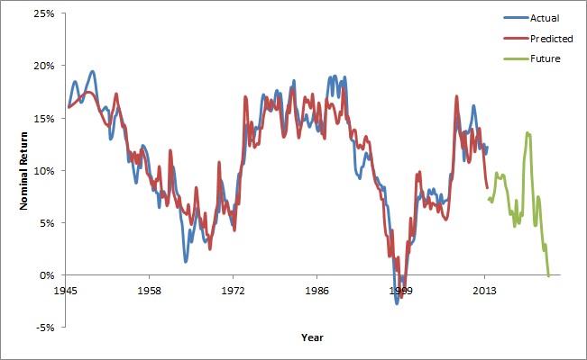
The fit is now even better that just equity allocation of investors alone with a correlation coefficient that has improved from about 0.903 R2 to 0.935 R2. That may not seem like much to you, but the variance in the data has been reduced by about 32% over the previous measure! Figure 6 plots the residuals of this data.
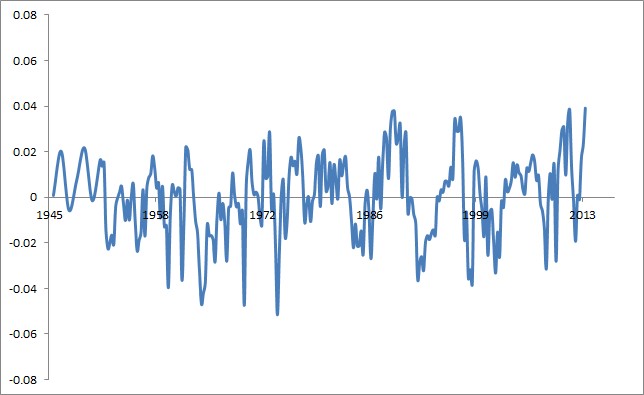
As you can see, the residuals now no longer have a systematic curvature to them, but instead look like flat random noise. Further, we have reduced the maximum range of errors from about +/-6% to about +3.8%/-5.1% with virtually all of the data points falling in the range of about +3% / -4%. This represents a substantial increase in the confidence intervals of our predictions.
Given that Figure 6 is now a flat, noisy baseline, we can have more confidence that we may have explained all of the possible sources of variance that are possible to explain with the model. In addition, this is still a simple, 2 parameter model – it only requires the equity allocation of investors and the inverse of treasury bond yields calculated above to predict future 10 year returns. Here is the new model of long-term market returns which inorporate anchored investor expectations about valuation:
Return = -0.7130 * EAI + 0.1198 * [1 / GS10]1 year average + 0.3254
where EAI is the current equity allocation of investors, and Return is the expected 10 year annualized total return on the S&P500.
Now, it should be said, that this model requires some time to validate, since there are no out of sample observations yet. There is still a chance that we have fit something which just by random chance happens to fit, and not because that is actually what is occurring. We will need to validate this model in the coming years to see. However, we have 2 things on our side in supporting that this model may be valid without having observed future data points yet. The first thing on our side is that we have used few parameters (only 2), and it is difficult to make data fit a simple model with over-fitting. It is usually obvious when this is being done also, since the model will contain a large number of complicated terms with the parameters in them. In other words, it won’t be very simple. If you can make a very simple 2 parameter model fit, without twisting and turning the data, there is a higher likelihood that it is describing the underlying phenomenon well. The second thing on our side is that we have constructed a model based on our understanding of the system and found it to be supported. If we had instead just fit 50 random parameters and tweaked everything using a computer to fit the model without understanding anything, we very likely could have something that fits all the existing data, but will fit none of the future data. This is because we overfit, and none of the many parameters we fit have a physical reason to be included in the underlying model, they just happened by chance to fit the noise. In our case, we have good reason to use the 2 parameters that we do, and we think we know why we have to fit those parameters to the return data in the way that we do based upon our understanding of the underlying system. Still, time will tell if we were correct or not.
Now that we have our new model in hand, I wanted to conclude with a discussion about future returns based on this model. I mentioned another blogger in the previous post, Aleph Blog, that periodically publishes his model updates for equity allocation of investors. This is the simpler version of the model, similar to the one that I introduced in the last post, one that contains no adjustments for anchoring of investor expectations, and only includes equity allocation of investors. Using that type of model, he (and I in the previous post on thestarinvestor.com) both mentioned that currently the model is predicting near 0% 10 year annualized future returns (in the case of my model it is 0.2% predicted returns as of the last equity allocation of investors published in Q1 2024). However, by incorporating anchoring expectations, we can see that returns are expected to even be a small bit lower than this at an annualized -0.1%. for the next 10 years on average.
I plan to periodically post updates on this model to see if it is still forecasting future long-term returns in the market accurately. I hope that it can be incorporated into models for future retirement planning and the like, if it proves accurate.
Leave a Reply