Using the Kelly criterion for sizing stock positions – Part 1

We have focused a lot on how to pick stocks and the idea of buy and hold. Now we should take a look at asset allocations and how much of our portfolio we should put into each stock. There will be a lot to talk about, so we will do this over the next two posts. To gain insights into how to size our allocations to various stocks, we can use the Kelly criterion to help us. The Kelly criterion is a mathematical formula originally developed for sizing bets where the gambler has an edge (i.e., over many bets, the gambler will on average make money).   By betting the amount of the Kelly bet each time, the gambler will avoid ruin and maximize the rate of growth of his or her bankroll over time.  If the gambler has no edge, the Kelly criterion recommends no bet, and if the edge is negative, the Kelly criterion recommends taking the other side of the bet (which is not always possible, since, for example, a casino will not let you be the house while it takes the risky bet).

In the most naïve sense, stocks can also be looked at as bets with completely random win or lose outcomes like gambling.  They can have winning edges also.  Therefore, we can utilize the Kelly criterion to size bets (i.e., allocate a fraction of our total portfolio value to an individual stock).  First, let’s take a look at the formula for the Kelly criterion.  The bet size for a given round of betting is given by:

f = p – (1-p)/b

Here, f is the fraction of the bankroll or portfolio value to wager, p is the probability of a win (so 1-p is the probability of a loss), and b is the proportion of the bet gained with a win divided by the amount lost with a loss.  To calculate b, you calculate the amount won for a winning bet (not the bet itself), and divide by the amount lost for a losing bet.  It is the odds expressed as a decimal fraction.  Here are a few examples to illustrate:

Example 1:

If you pay $100 to bet and you will receive $200 back if you win ($100 original bet + $100 in winning profit), and 0 back if you lose, then b is 1 ($100 profit if you win / $100 bet lost if you lose = 1).  Your probability of winning is 60% (p=0.6), therefore your probability of losing is 40% (1-p = 0.4).  The Kelly criterion says your bet size should be f = 0.6 – (1-0.6)/1 = 0.2, or a bet size of 20% of your portfolio.  Note that this outcome has a positive expected gain (0.6 * 2 – 0.4 * 0 = 1.2, i.e, you have a 20% gain on average over many bets).  The Kelly Criterion will only tell you to make a bet when there is a positive expected gain.  It will give you a negative value if there is a negative expected gain (i.e., you should take the other side of the bet) and it will give you a value of 0 (no bet) if there is no edge for either side of the bet.

Example 2a:

You buy a stock and it has an average probability of winning of 50%, and an average probability of losing of 50%.  If you win, you make 100% on average, and if you lose, you lose 50% on average.  p = 0.5, b = 1/0.5 = 2.  The Kelly bet (stock allocation) is f = 0.5 – (1-0.5)/2 = 0.25 or 25% of your portfolio.

The Kelly criterion makes a couple of assumptions that are important to know about:

1. Bankroll is infinitely divisible.  So for example, if the bankroll becomes arbitrarily small, you can always bet a fraction of that.  In reality, this is not the case.  If you only have 1 penny of your bankroll left, you can’t usually divide it into tenths and then purchase 10 different stocks with it.  So there is a practical limitation, but we will avoid this issue with a trick in the discussion below.
2. There is a binary outcome – either a win or a loss with fixed rules for each outcome.  This is not the case for stocks – there can be different probabilities of earning a 100% return vs. a 10% return, and the same is true for losses.  In fact there is a distribution of probabilities of each range of returns.  This can be overcome by using an average expected win or loss amount and an average expected win or loss probability, with some important caveats which we will discuss below.
3. This binary outcome assumes total loss for a loss, and a set amount for a win.  Generally for gambling scenarios, you lose the entire amount of a bet when you lose, but for stocks you most often will only have a partial loss.  We will discuss below when and why we can violate this assumption.
4. This formula does not account for volatility.  By volatility, I mean from the perspective of your portfolio growth/shrinkage with each bet, not the volatility of the stock itself.  Although these 2 types of volatilities are linked together, they are different.  Volatility of the stock is actually addressed in point 2 above, where the distribution of win and loss returns is discussed.  Addressing portfolio volatility, the win/loss ratio, b, is the same for a stock with a possible gain of 300% and a loss of 100% as it is for a stock with a possible gain of 3% and a loss of 1%.  However, a stock delivering gains and losses in the former case will cause a much more volatile set of ups and downs in your portfolio as you make each bet.  This will be addressed below.
5. The outcomes are completely known beforehand.  For games of chance, one can often know based on the rules, what the probability of winning and losing is, and exactly how much one will win or lose in each case.  Stocks are less well defined, particularly for individual stocks where unknown events can affect outcomes.  This lessened to a degree with large averages of stocks, such as the S&P500 index, but it is not completely removed from consideration.
6. The final assumption for the Kelly criterion that is important is that it is a singular event based bet.  A bet is one event that happens and is then finished, so there is not an element of time to it.  For stocks, holding period matters, so the event can change based on how we define the holding period.  We will deal with this assumption in the next post. 

Now, if you notice, in Example 2a, we violated one of the assumptions of the Kelly criterion formula (assumption 3).  We assumed that with a stock investment, there was only a partial loss, while this version of the formula for the Kelly criterion assumes total loss in the event of a losing situation.  We know that total losses for individual stock investments are not common (hopefully).  Therefore, a more accurate form of the Kelly criterion for partial losses is:

f = p/L + (1-p)/W

Where f and p are as defined before, L = fraction that is lost in when a loss occurs, W = fraction that is won when a win occurs.  Let’s look at Example 2a again, but calculated instead with this version of the formula:

Example 2b:

You buy a stock and it has an average probability of winning of 50%, and an average probability of losing of 50%.  If you win, you make 100% on average, and if you lose, you lose 50% on average.  In this case p = 0.5, W = 2-1/1 = 1, L = 1-0.5/1 = 0.5, and the Kelly criterion tells you that you should bet f = 0.5/0.5 – (1-0.5)/1 = 0.50 or 50% of your portfolio each time you have a chance to make a bet like this.

Notice that with this version of the formula, the Kelly criterion predicts a bet size that is a much larger fraction of your portfolio than the version which assumes total loss.  This makes sense, because the loss is not total for a losing bet in this case.

This version of the Kelly criterion also takes into account portfolio volatility.  Let’s look at another example:

Example 2c:

You buy a stock and it has an average probability of winning of 50% and an average probability of losing of 50%.  If you win you make 10% on average, and if you lose, you lose 5% on average.  This is a much less volatile example than in the situation presented in Examples 2a and 2b, but with the same probability of a win or loss.  When using the first version of the Kelly criterion, b is the same (b = 10% gain if win / 5% loss if losing = 2), so the first version of the Kelly criterion predicts the same bet size as in Example 2a, f = 0.5 – (1-0.5)/2 = 25%.  However, the second version of the formula which takes into account partial losses, predicts a very different situation.  For that case, p = 0.5, W = 1.1-1/1 = 0.1, L = 1-0.95/1 = 0.05, and f = 0.5/0.05 – 0.5/0.1 = 5.  This version of the Kelly criterion predicts a number bigger than 1, so it is actually telling you to leverage your portfolio 5x and make the bet to maximize the return.  This second version of the Kelly criterion will often give values greater than 1 (i.e., make a bet that is bigger than your portfolio size by levering up) for situations where the bets do not swing portfolio values very widely.

Example 2c actually illustrates a serious problem with the second version of the Kelly criterion, which was brought up in point 2 of the list of assumptions above.  We don’t actually have a binary outcome, we have a probability distribution of outcomes for a stock.  Taking the example scenario of 2c above, if you were to lever up your portfolio 5x because you assume a binary outcome (either a 10% gain or a 5% loss), and you instead actually lose 20%, your portfolio experiences a complete loss (5 * 20% = 100%).  The Kelly criterion is designed precisely to avoid total run, but it has instead led you to make a bet that sooner or later will almost certainly lead to total ruin due to violation of a critical assumption.

There are some strategies to avoid this, however.  In general, I think you should use the first version of the Kelly criterion, even for situations of partial loss, because it gives more conservative estimates.  You should also consider worst case scenarios in your range of calculations to avoid making a bet size that is too large.  There is also an extremely useful tool, called making a half Kelly bet.

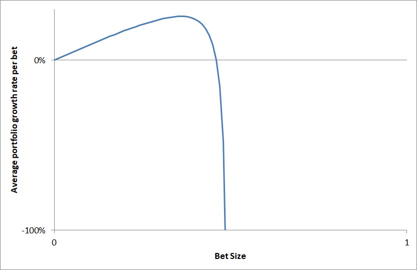
The half Kelly bet arose because of an issue outlined in assumption 5 above.  The outcome of the Kelly betting is based on precisely known win and loss rates and betting odds.  For simple games of chance, these parameters can be precisely known, but for many other situations, it can be difficult to accurately estimate precise amounts.  Further, small errors in these estimates can lead to total ruin, which the Kelly criterion is supposed to prevent.  It was noticed that Kelly bets followed a distribution that roughly looks like the one shown in Figure 1.  For bets that are smaller than the Kelly bet, the growth rate slowly improves until you reach the Kelly sized bet, which has the maximum growth rate.  Then, if you over-bet the Kelly sized bet by increasing amounts, the portfolio growth rate begins to rapidly decline and very quickly leads to a bet size where total ruin of the portfolio is certain over many bets.  It was noticed that a value of ½ the Kelly bet does not lead to too much reduction in growth rate, but takes you far away from this cliff where potential ruin can occur with small errors in estimating win and loss rates and betting odds.  Therefore, it is generally agreed that you should make a bet of ½ the size of the Kelly bet in cases where the situation is not perfectly known.  It is more important to avoid total ruin than to squeeze the last small bit of growth out of the average bet.

The ½ Kelly bet takes care of problems with several assumptions made in the list above.  First, it reduces the need for an infinitely divisible bankroll/portfolio, because your bet size should be very far from taking your bankroll to very small sizes (i.e., dangerously close to total ruin).  Second, it makes the formula much safer to use for situations that are not precisely known.  Third, for stocks, where there is actually a distribution of return outcomes it makes your bet size much safer.  You can use an average win or loss rate, and an average win/loss odds without having to worry about very extreme outliers leading you to total ruin because you did not use a more detailed model with a probability distribution of outcomes.  Like the Gordon growth model discussed previously, the Kelly criterion is more of a very quick way to estimate scenarios and get a feel for the behavior of things rather than an exact solution to an imprecise problem.  In addition, it is a very simple formula you can quickly calculate, as opposed to needing to run a computational simulation with a full probability distribution.

When using the Kelly criterion to estimate bet sizes or stock allocations, observe the following rules:

1. Always use the first, more conservative version of the formula as defined above, even when partial losses are the probable outcome in losing scenarios.
2. Always use a ½ Kelly bet or stock allocation size as it will not reduce growth much from the optimum but will make the allocation much safer in the case of small errors in estimation of win and loss rates and betting odds, as well as reduce errors from the fact that stocks do not produce binary outcomes, but instead have a probability distribution for outcomes.
3. Never go above 50% to any one stock (we will define further what the Kelly criterion says about stock allocations in the next post, and reduce this more based on historical stock data).
4. Never leverage your portfolio if the Kelly criterion is telling you to make a bet with size larger than f = 1.  This goes for stock indices as well.  For indices, which are averages of many stocks, never go above f = 1 (which is a leveraged position).

Now we can start to look at allocations to different stocks based on the conviction that you have about them.  For example, let’s say that you allocate 5% of your portfolio to a stock.  What does that say about how much you believe the stock will deliver a win vs. a loss?

Example 3:

Let’s say that you allocate 5% of your portfolio to a winning stock.  The average winning stock that you pick in your portfolio gives a 20% return, and the average losing stock that you pick gives a 10% decline in your portfolio value (so b = 20%/10% = 2).  f = p – (1-p)/2 = 0.05.  Solving for p we get p = 36.67%.  In other words, you are implying that you think there is a 36.67% chance of winning, and a 63.33% chance of losing on such a trade.

You can also use this to size your positions to a degree based on your conviction for a trade.  Conviction should be relative to the other things you hold in your portfolio, so a high degree of conviction says you believe that it has a better chance of winning than most other stocks in your portfolio.

Example 4:

Let’s say that you have a high degree of conviction on a trade.  Your portfolio typically delivers a win rate of 50%, and the typical win is for a 30% gain while the typical loss is 20%.  Your high conviction trade means you estimate p = 0.6 (i.e., a 60% win rate which is above your normal rate of 50%), and you estimate a similar gain for wins and shrinkage for losses as is typical for your portfolio (b=30%/20% = 1.5).  Therefore, f = 0.6 – (1-0.6)/1.5 = 0.3333, and a full Kelly bet would be 33.33%, so you use the ½ Kelly bet value of 16.67%.

Now that we have laid the groundwork for understanding the Kelly criterion, we will be able to use it to get an idea of stock allocations in our portfolio.  A few realistic example use cases were presented (Examples 3 and 4).  In the next post, we will look at using the Kelly criterion to tell us about maximum allocation to any one stock, as well as how holding time plays a role in the outcome of a stock trade.